Appendix 3: Deriving the Knowability Map
Appendix 3 to AGI: How Superhuman Intelligence Reshapes Civilization. Documents the assumptions, calculations, interpretation, and limits of the Knowability Map introduced in Chapter 8.
Last updated: September 14, 2026 (JST)
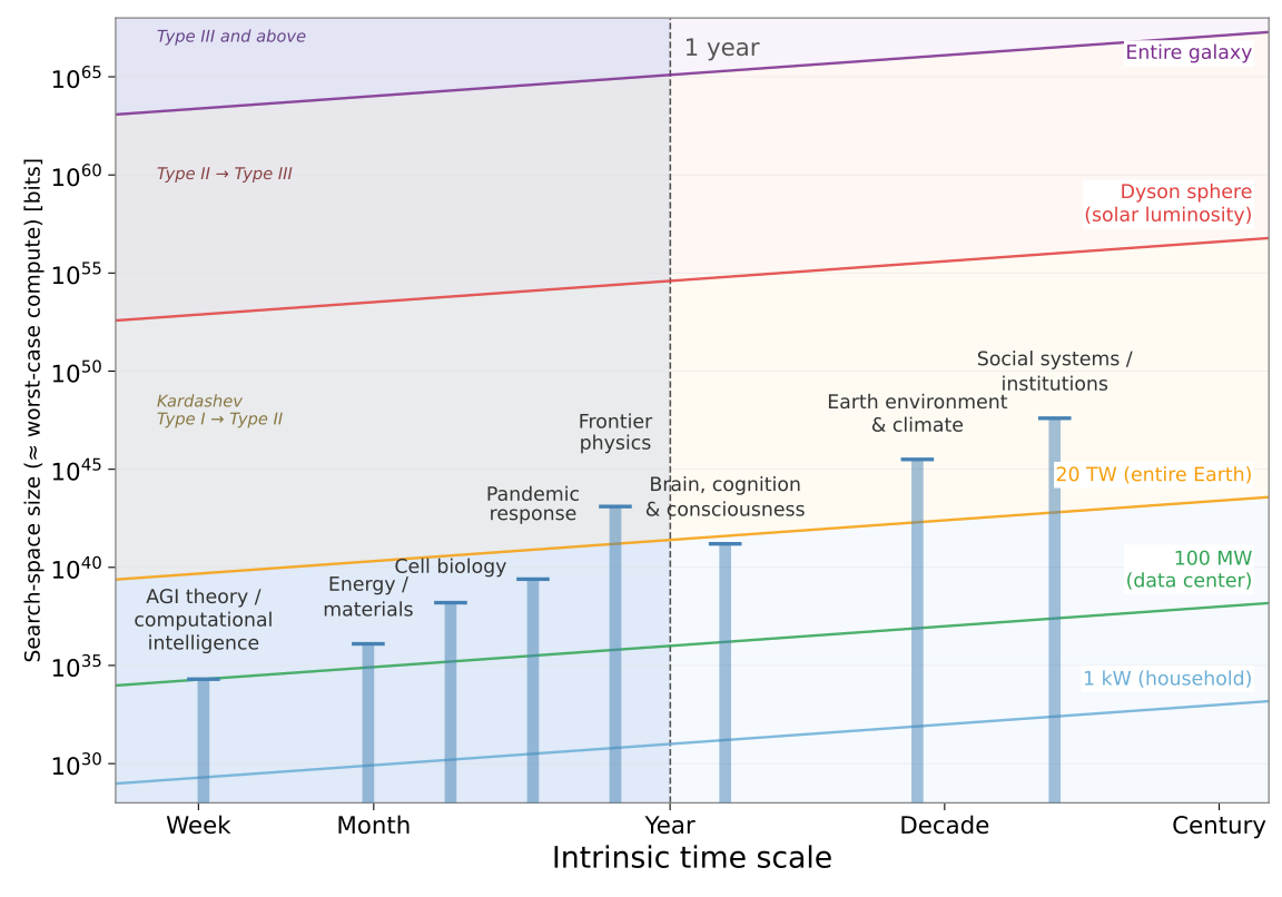
In Chapter 8 we introduced the "Knowability Map," which assesses the scientific frontier reachable by AI-driven science under three constraints: (1) the intrinsic timescale of the target system, (2) the required amount of computation, and (3) the energy that can be supplied. This appendix sets out the premises behind that figure, the numerical settings for each problem group, the calculation of the energy tiers, how to read the figure, and its limitations.
Appendix 3 — Contents
- Aim of the figure — axes and display units
- Basic premises — A: irreversible computation / B: waiting time / C: interval assessment
- What the bars mean — the interval and the basis for its upper end
- Why bars rather than points — the effect of this representational choice
- Why the upper end is $2^{K_{\mathrm{eff}}}$ — the basis for the Levin upper bound
- Problem groups and intrinsic timescales — placement table for the eight problem groups
- Energy tiers — five tiers from 1 kW to an entire galaxy
- Testing one-year reachability — the time condition and the computation condition
- Main conclusions readable from the figure — reachability by tier
- Limitations of this figure — six caveats
- Basis for the settings of each problem group — the $K_{\mathrm{eff}}$ breakdown and the specific circumstances of the eight problem groups
- How to read these sections — the convention for assigning bits, and natural cycles per year
- AGI theory and computational intelligence — $t=10^{5.8}$ s, $K_{\mathrm{eff}}=114$
- Energy and materials — $t=10^{6.4}$ s, $K_{\mathrm{eff}}=120$
- Cell biology — $t=10^{6.7}$ s, $K_{\mathrm{eff}}=127$
- Pandemic response — $t=10^{7.0}$ s, $K_{\mathrm{eff}}=131$
- Frontier physics — $t=10^{7.3}$ s, $K_{\mathrm{eff}}=143$
- Brain, cognition, and consciousness — $t=10^{7.7}$ s, $K_{\mathrm{eff}}=137$
- Earth environment and climate — $t=10^{8.4}$ s, $K_{\mathrm{eff}}=151$
- Social systems and institutions — $t=10^{8.9}$ s, $K_{\mathrm{eff}}=158$
- Supplementary notes on the overall layout — contrasting the characteristics of the eight problem groups
Aim of the figure
The Knowability Map organizes scientific problems along the following axes.
- Horizontal axis: intrinsic timescale of the target system [seconds]
- Left vertical axis: required amount of computation $C_{\mathrm{req}}$ [bit erasures at 300 K]
- Right vertical axis: effective Kolmogorov complexity $K_{\mathrm{eff}}$ [bits]
The $K_{\mathrm{eff}}$ of the right vertical axis is the scale obtained by re-reading the left axis through $C = 2^{K_{\mathrm{eff}}}$; it serves to read the height of a bar's upper end as an exponent.
On this basis, it visualizes the "scientific frontier reachable within one year" for each level of energy input. The energy tiers are taken in five steps: 1 kW (an ordinary household), 100 MW (a giant data center), the entire Earth (humanity's total primary energy consumption, approx. 20.6 TW), a Dyson sphere (1 $L_\odot$), and an entire galaxy. The use of this figure lies in allowing three constraints — energy, search computation, and the time of the target system — to be compared intuitively on one and the same plane.
Each problem group is represented not by a single point but by a "vertical bar": an interval whose lower end is the information-theoretic lower bound $O(K_{\mathrm{eff}})$ and whose upper end is the Levin search upper bound $O(2^{K_{\mathrm{eff}}})$, and whose length represents the margin that is required in principle but can be compressed by algorithmic improvement.
Basic premises
Premise A: AGI can perform irreversible computation near the Landauer limit
We take the minimum energy required to irreversibly erase one bit to be
$$ E_{\mathrm{bit}} = k_B T \ln 2 $$
At 300 K this gives
$$ E_{\mathrm{bit}} = 1.380649 \times 10^{-23} \times 300 \times \ln 2 \approx 2.87 \times 10^{-21},{\mathrm{J/bit}} $$
Accordingly, for power $P$ over duration $\tau$, the maximum amount of computation that can be supplied is
$$ C_{\max}(P, \tau) = \frac{P,\tau}{k_B T \ln 2} $$
Premise B: The engineering waiting time of experiments is zero
We assume that sample preparation, application of perturbations, measurement, data retrieval, and generation of the next experimental condition are all automated and take negligible time. The only time that therefore remains on the horizontal axis is the intrinsic physical, biological, or social timescale possessed by the target system itself.
Premise C: The required amount of computation is assessed as an interval
Rather than fixing the required amount of computation for each problem group at a single point, we represent it by the following interval.
If the essential shortest description length of the problem is $K_{\mathrm{eff}}$ bits, then at least information processing of that order is required (the lower end, the information-theoretic lower bound).
$$ C_{\mathrm{low}} \sim K_{\mathrm{eff}} $$
If the shortest program length is $K_{\mathrm{eff}}$, we take the following as the upper bound of universal search — Levin search, which tries all possible programs in parallel, from the shortest upward (the upper end, the Levin search upper bound).
$$ C_{\mathrm{high}} \sim 2^{K_{\mathrm{eff}}} $$
What the bars mean
Why bars rather than points
A point representation makes it look as though "the required amount of computation is uniquely determined," but in reality, even for the same problem, the required amount of computation varies greatly depending on
- whether a good representation can be found
- whether a good modeling scheme can be found
- whether the causal structure can be made explicit
- whether an efficient search algorithm can be discovered
For this reason, representing the required amount of computation as a range from $K_{\mathrm{eff}}$ to $2^{K_{\mathrm{eff}}}$ is closer to the essence of scientific problems.
- Bottom of the bar = below this, it is impossible in principle
- Top of the bar = compute this much and it is theoretically guaranteed to be reachable
- The middle of the bar = determined by the quality of algorithms, the discovery of representations, and the skill of experimental design
Note that the information-theoretic lower ends — $K_{\mathrm{eff}}$ of 114–158 bits, or on the order of $10^{2}$ when converted into computation — lie far below the vertical range of the chart (which starts at $10^{28}$) and are therefore not shown in the figure. Each bar is drawn rising from the bottom edge of the axes and should be read as continuing downward beyond the chart.
Why the upper end is $2^{K_{\mathrm{eff}}}$ (search computation, not representation size)
Naively, one is tempted to estimate the required amount of computation as "the size of the representation of the knowledge finally obtained." For example, even 1 kW × 1 year permits information processing on the order of $10^{31}$ bits, and on that measure many problems would look "theoretically feasible."
In this figure, however, we distinguish:
the size of a knowledge representation ≠ the search computation needed to discover that knowledge
The difficulty of discovery is determined not by the length required to write down the knowledge obtained, but by the size of the hypothesis space that must be searched in order to reach that knowledge.
We therefore adopt the Levin-type $2^{K_{\mathrm{eff}}}$ as the upper bound on search cost. The figure is drawn as an interval: the lower end $K_{\mathrm{eff}}$ is a theoretical lower bound close to representation size, and the upper end $2^{K_{\mathrm{eff}}}$ is a theoretical upper bound that includes search.
This figure is therefore not a diagram of knowledge storage capacity, but "an upper-bound diagram that includes the search difficulty of scientific discovery."
Problem groups and intrinsic timescales
The horizontal position of each problem group is fixed at an approximate value of the intrinsic timescale of the target system. Vertically, the lower end is $K_{\mathrm{eff}}$ and the upper end is $2^{K_{\mathrm{eff}}}$. Taking one year as $3.15\times 10^7$ seconds, the number of natural cycles that can be observed or intervened upon per year is also listed. For the breakdown of the $K_{\mathrm{eff}}$ value of each problem group and its specific circumstances, see Basis for the settings of each problem group.
| Problem group | Intrinsic timescale [seconds] | $\log_{10}(t)$ | $K_{\mathrm{eff}}$ [bits] | Upper end $\log_{10}(C_{\mathrm{req}})$ | Natural cycles per year |
|---|---|---|---|---|---|
| AGI theory and computational intelligence | $10^{5.8}$ | 5.8 | 114 | 34.3 | about 50 |
| Energy and materials | $10^{6.4}$ | 6.4 | 120 | 36.1 | about 13 |
| Cell biology | $10^{6.7}$ | 6.7 | 127 | 38.2 | about 6 |
| Pandemic response | $10^{7.0}$ | 7.0 | 131 | 39.4 | about 3 |
| Frontier physics | $10^{7.3}$ | 7.3 | 143 | 43.1 | about 1.6 |
| Brain, cognition, and consciousness | $10^{7.7}$ | 7.7 | 137 | 41.2 | about 0.6 |
| Earth environment and climate | $10^{8.4}$ | 8.4 | 151 | 45.5 | about 0.13 |
| Social systems and institutions | $10^{8.9}$ | 8.9 | 158 | 47.6 | about 0.04 |
Energy tiers
Each diagonal line represents the maximum amount of computation that can be supplied when a given power $P$ is used for one year.
$$ \log_{10} C_{\max}(t) = \log_{10} C_{\max}(1,{\mathrm{yr}}) + \log_{10}!\left(\frac{t}{1,{\mathrm{yr}}}\right) $$
That is, on a logarithmic plot it becomes a straight line of slope 1.
| Energy tier | Power $P$ [W] | Maximum computation in one year $\log_{10}(C_{\max})$ |
|---|---|---|
| 1 kW (an ordinary household) | $10^{3}$ | 31.0 |
| 100 MW (a giant data center) | $10^{8}$ | 36.0 |
| The entire Earth (approx. 20.6 TW) | $2.06\times10^{13}$ | 41.4 |
| A Dyson sphere (1 $L_\odot$) | $3.83\times10^{26}$ | 54.6 |
| An entire galaxy | $1.15\times10^{37}$ | 65.1 |
The values in the table are totals for one year. The value at the intrinsic-timescale position, which the test below (Condition 2) uses, is this value minus $\log_{10}(1,\mathrm{yr}/t)$. For example, reading the 100 MW diagonal at the position of AGI theory and computational intelligence, $t=10^{5.8}$ seconds, gives $36.0-1.7=34.3$.
In addition, a vertical dashed line for "one year" is drawn at the position $t = 10^{7.5},{\mathrm{s}}$. The background colors of the figure correspond to the Kardashev scale, a classification of civilizations by the total energy they can harness (Type I planetary, Type II stellar, Type III galactic). The band between the diagonals for the entire Earth and a Dyson sphere marks the transition from Type I to Type II, and the band between a Dyson sphere and an entire galaxy the transition from Type II to Type III.
Testing one-year reachability
For a given problem group to be reachable within one year at a given energy level, there are two conditions.
Condition 1: The time condition
The horizontal position of the problem group must lie to the left of the one-year vertical dashed line.
$$ t_{\mathrm{intrinsic}} \le 1,{\mathrm{year}} $$
Condition 2: The computation condition
The top of the problem group's bar must lie below the diagonal line for that energy level. Because each diagonal represents, with slope 1, the cumulative computation that can be supplied up to duration $t$, the height of the diagonal is read at the bar's horizontal position — that is, at the intrinsic timescale of the target system. It is read at the intrinsic-timescale position because the result of a search is tested by one response of the target system. Computation that cannot exhaust its candidates within one cycle is not in time for that round's experiment and is carried over to the next cycle. The computation used in the test is therefore not the total for one year but the amount that can be supplied during one cycle. The one-year condition operates separately, on the side of Condition 1, as the question of whether that one cycle fits within a year.
$$ C_{\mathrm{high}} \le C_{\max}(P, t_{\mathrm{intrinsic}}) $$
When both conditions are satisfied, the problem is reachable within one year even on the Levin upper bound — that is, it lies in the "assuredly reachable region."
If, on the other hand, the top of the bar is above the diagonal, the problem is still reachable information-theoretically — the lower end lies far below the diagonal — but whether it is actually reached depends on the discovery of algorithms and representations.
Main conclusions readable from the figure
Reading each energy tier's diagonal at the horizontal position of each bar gives the following.
- 1 kW (an ordinary household): On a within-one-year, Levin-upper-bound basis, no problem group is reached. The smallest gap between the diagonal and a bar top is the roughly 5 orders of magnitude of AGI theory and computational intelligence; whether that gap can be closed depends on the discovery of algorithms and representations.
- 100 MW (a giant data center): The upper end of AGI theory and computational intelligence is very nearly reached; at the bar's horizontal position of $10^{5.8}$ seconds, the height of the diagonal is $10^{34.3}$, coinciding with the upper end. For energy and materials, the diagonal stops about 1.2 orders of magnitude below the upper end — short of assured reachability, but near the boundary on a figure whose vertical axis spans 40 orders of magnitude. From cell biology onward, the upper end is still too high.
- The entire Earth (approx. 20.6 TW): The upper ends of AGI theory and computational intelligence, energy and materials, cell biology, and pandemic response fall below the diagonal and come within one-year reach. Frontier physics still has its upper end about 1.9 orders of magnitude above the diagonal, so the computational wall remains. Brain, cognition, and consciousness has its upper end below the diagonal, but its intrinsic time exceeds one year. For climate and social institutions, the upper end still lies more than 3 orders of magnitude above the diagonal, and the intrinsic time is decisively long besides.
- A Dyson sphere ($1,L_\odot$): The computational constraint almost vanishes. Nevertheless, problems with long intrinsic times, such as climate and institutions, still cannot be settled within one year.
- An entire galaxy: The computational constraint becomes entirely secondary. The wall that remains to the very end is "the time the target system takes to advance on its own."
Limitations of this figure
This figure is strictly an upper-bound assessment, not a prediction, and its limitations are many.
- $K_{\mathrm{eff}}$ is not a rigorous Kolmogorov complexity but a proxy quantity for the effective search complexity of each problem group
- The constant factors of Levin search are enormous, so it is not usable in practice
- The very assumption of computation near the Landauer limit is extremely optimistic
- Communication, error correction, memory access, experimental failure rates, and observational noise are ignored
- In social-institutional systems, the "reflexivity" whereby observation is altered by intervention is strong, making simple reduction to a timescale difficult
- Even within the same problem group, $K_{\mathrm{eff}}$ can change greatly through the discovery of a representation
Basis for the settings of each problem group
How to read these sections
Below, we record the approximate basis for the two quantities that determine each problem group's vertical bar: the intrinsic timescale $t$ of the target system, and the effective Kolmogorov complexity $K_{\mathrm{eff}}$.
$K_{\mathrm{eff}}$ here is not the amount of information required to describe the target completely (for cell biology, the entire genome sequence or all single-cell data; for climate, every observational grid point; for social institutions, the histories of every individual), but the effective description length needed to describe, taken together, the minimal mechanistic model required to make the problem group in question "knowable" — that is, the hypothesis class, the governing variables, a coarse specification of precision, the observation map, and the intervention map.
The assignment of bits follows the following convention. $4$ bits corresponds to a coarse selection among roughly $16$ types, $8$ bits to a discretization of roughly $256$ levels, $12$ bits to some thousands of combinations, and $16$ bits to a coarse structural selection among some tens of thousands. Accordingly, the numbers below are not "precise values in bits" in the sense of significant figures; they are minimum-description-length (MDL) style rules of thumb for positioning the relative search difficulty across problem groups. They must be read not as reproducible measurements but as working calibration values for explaining the relative layout of the figure.
Conversion into years is an indicative aid for display only; below, the second values and $\log_{10} t$ given in the tables are treated as the primary values. The number of natural cycles per year, converted by taking one year as $3.15\times 10^7$ seconds, is listed in the table under Problem groups and intrinsic timescales.
This cycle count gives the intuitive meaning of the horizontal axis in the Knowability Map. In problem groups where the target system responds dozens of times within a year, the effects of AGI-driven theoretical search, experimental planning, and model revision can readily appear iteratively. Conversely, in problem groups such as climate or institutions, where the target system does not complete even one full turn within a year, the verification cycle in the real world itself becomes rate-limiting, however powerful the AGI.
AGI theory and computational intelligence
Values adopted: $t=10^{5.8}$ s, $K_{\mathrm{eff}}=114$ bits
Intrinsic timescale
The representative process adopted is "one full turn of the computational-intelligence research cycle of theoretical hypothesis, implementation, evaluation, counterexample generation, and revision." The target system here is taken to be not a single inference pass of a single neural network, but "the hypothesis space of computational structures that give rise to intelligence." That is, the representative value is the shortest effective cycle from giving a certain learning rule or agent configuration, through its changing behavior on a task set and returning failure cases, to the next hypothesis being formulated from those failure cases.
The value of $10^{5.8}$ s — about one week — means that the AGI problem group is placed on the shortest-timescale side of this map. This is because the target is artificial, symbolic, and simulable, and does not necessarily have to wait on natural time such as material synthesis, cell culture, epidemic spread, climate response, or institutional change.
Three candidates were not adopted. First, single-inference times of milliseconds to seconds. This is correct as the output response of a language model or policy model, but it is not the time constant on which "AGI theory is revised." Second, large-scale training runs of weeks to months. This depends too heavily on computational resources, implementation, and the distributed-training environment, and readily includes setup time that Premise B should exclude. Third, the year-scale timescale corresponding to human education and development. This is a constraint of biological cognition and is too long for the intrinsic timescale of computational intelligence in general.
From the standpoint of one-year reachability, AGI theory and computational intelligence has about 50 cycles. This means that, within the same hypothesis class, there is ample room for an AGI to generate failure cases, revise the model, and re-evaluate. At the same time, a timescale of one week does not merely mean "fast": because the evaluation criteria themselves change, models game the evaluation, and the search process becomes self-referential, the shorter the cycle, the greater the danger of Goodharting (evaluation breaking down as the metric is gamed) and overfitting.
Decomposition of $K_{\mathrm{eff}}$ into degrees of freedom
| Degree of freedom | bits | Basis for the assignment |
|---|---|---|
| Problem/task set and success criteria | 15 | Coarsely specifies combinations of prediction, control, dialogue, long-horizon planning, self-revision, and so on. A selection among roughly $2^{15}$ task families. |
| Representation space and state abstraction | 14 | Specifies the encoding schemes for tokens, images, actions, memory, world state, and latent variables. |
| Learning, search, and update dynamics | 16 | Combinations of gradient learning, reinforcement learning, Bayesian updating, search, self-supervised learning, and meta-learning. |
| Architectural primitives and composition grammar | 13 | Composition rules for attention, recurrence, external memory, modularization, tool use, and so on. |
| Planning, credit assignment, and search control | 11 | Coarse specification of long-horizon rewards, delayed rewards, counterfactual reasoning, and search depth. |
| Memory, world model, and environment interface | 12 | Short-term memory, long-term memory, external tools, and maps for environment-state updating. |
| Alignment and control constraints | 11 | Coarse description of goal stability, instruction following, safety constraints, and self-modification constraints. |
| Scaling laws and normalization of computational resources | 8 | Coarse exponents and thresholds of performance curves with respect to data volume, model size, and computation. |
| Evaluation and observability model | 8 | Observation maps for benchmarks, dialogue evaluation, behavioral evaluation, and counterexample generation. |
| Abstraction priors and invariances | 6 | Minimal prior assumptions such as compositionality, causality, compressibility, and symmetry. |
| Total | 114 |
Specific caveats
The $K_{\mathrm{eff}}$ of this problem group is comparatively small not because AGI is easy, but because artificial computational systems are, compared with matter, life, and society, observable, reproducible, and easy to compress symbolically, so that the description length of the minimal mechanistic model can be estimated to be relatively short.
Even so, the search upper bound remains large. In AGI, the object to be solved includes the searching agent itself. That is, the model predicts the evaluation, games the evaluation, and changes the meaning of the evaluation. The difficulty here is therefore concentrated not in long time constants of the external world, but in self-reference, the reflexivity of evaluation, and the instability of goal specifications.
Energy and materials
Values adopted: $t=10^{6.4}$ s, $K_{\mathrm{eff}}=120$ bits
Intrinsic timescale
The representative process adopted is "one full turn of the closed-loop materials-search cycle of synthesis of candidate materials, structural relaxation, property evaluation, detection of signs of degradation, and model updating." Concretely, for battery materials, catalysts, photovoltaic materials, thermoelectric materials, structural materials, and the like, we take as representative the natural response time from making a candidate composition, measuring it, coarsely confirming its performance and stability, and moving on to the next candidate.
This value is not a microscopic time constant such as an electronic transition or a phonon response, but the time until the material responds as a "useful macroscopic property." In materials development, even though the quantum-mechanical description is extremely compact, what one actually wants to know are effective properties that include defects, phase separation, interfaces, grain boundaries, degradation, and fabrication conditions. The Materials Genome Initiative, a United States national program launched in 2011 to accelerate materials development, sets out to integrate data, models, simulation, and standardization in order to reduce the time and cost of discovering, optimizing, and deploying materials1. In materials science, closed-loop search combining such data infrastructure with automated experimentation and active learning is positioned as a framework for accelerating the discovery of molecules, materials, and systems.
Candidates not adopted are, first, electronic and molecular motion on femtosecond-to-nanosecond scales. This is intrinsic in physical terms, but it is not the rate-limiting factor determining the knowability of the materials problem group. Second, the time of a single synthesis or a single calculation. This is the processing time for one candidate, not the response time of a materials problem that includes properties, stability, and manufacturability. Third, the year-to-decade timescale of commercialization, mass production, and market introduction. This includes too much of the time of technological systems, institutions, and industrial investment, so it is not treated here as a social-implementation time constant.
From the standpoint of one-year reachability, about 13 closed-loop search cycles are possible. Accordingly, if the hypothesis space is sufficiently compressed, measurement is automated, and failure data accumulate, the probability of discovering promising material candidates within one year is high. On the other hand, for problems involving long-term stability and degradation under real-world conditions, evaluation on a one-month cycle is no more than a shortened proxy indicator, and genuine lifetime prediction requires extrapolation.
Decomposition of $K_{\mathrm{eff}}$ into degrees of freedom
| Degree of freedom | bits | Basis for the assignment |
|---|---|---|
| Composition, element families, and chemical space | 18 | Coarsely specifies combinations of elements, stoichiometry, dopants, and substitution series. |
| Crystal structure, phases, and microstructure | 16 | Coarse structural types such as symmetry, phase separation, grain boundaries, defects, and amorphicity. |
| Electronic, thermodynamic, and transport descriptors | 14 | Effective descriptors such as band structure, free energy, diffusion, and conductivity. |
| Synthesis process variables | 15 | Discretization of temperature, pressure, solvent, precursors, calcination, film deposition, and cooling history. |
| Operating environment and boundary conditions | 12 | Use environments such as electrical potential, temperature, humidity, irradiation, and mechanical stress. |
| Target properties and trade-off functions | 12 | Multi-objective optimization over efficiency, capacity, stability, cost, safety, and so on. |
| Surrogate models and active search policies | 15 | Bayesian optimization, physics-constrained ML, and schemes for coupling with first-principles calculations. |
| Degradation, failure, and rare failure modes | 10 | Coarse classification of failures such as corrosion, interfacial fracture, phase transitions, and side reactions. |
| Measurement calibration and scale transfer | 8 | Maps from small samples to devices, and from devices to real environments. |
| Total | 120 |
Specific caveats
In energy and materials, the fundamental equations themselves can be written comparatively briefly. The problem lies in the fact that practical properties are not simple functions of microscopic states but are determined by synthesis history, defects, interfaces, environment, and degradation processes.
$K_{\mathrm{eff}}$ is therefore not the description length of quantum mechanics but the description length of "which coarse-grained variables must be retained in order to predict useful materials." There is no need to describe every atomic configuration, but one must choose which defects, which interfaces, and which degradation modes to retain as effective degrees of freedom. This choice is the difficulty specific to the materials problem group.
Cell biology
Values adopted: $t=10^{6.7}$ s, $K_{\mathrm{eff}}=127$ bits
Intrinsic timescale
The representative process adopted is "the multi-generational response by which a cellular state responds to a perturbation and transitions, via gene expression, signaling, metabolism, and epigenetic state, to a stable phenotype." The cell cycle of typical proliferating human cells is taken to be about 24 hours2, but here we adopt not a single cell division but the time until a reproducible change of state appears at the level of the cell population after a perturbation.
The value of $10^{6.7}$ s, about 58 days, encompasses on the order of several tens of cell cycles. This is because it includes not only the short-term response of gene regulatory networks but also selection, differentiation, reprogramming, cell–cell interactions, and phenotypic stabilization.
Candidates not adopted are, first, molecular reactions on the scale of seconds to minutes. These are the local time constants of enzymatic reactions and signal transduction, and do not represent the whole of the "problem to be solved" in cell biology. Second, the roughly one-day cell cycle. This is an important basic unit, but in many cases it is too short for a perturbation to be reflected in a stable cellular state. Third, the year-scale timescales of disease progression and organismal development. These go beyond cell biology and include too much of the time of tissues, organisms, the clinic, and the environment.
In the context of one-year reachability, there are about 6 natural cycles. Combining cell culture, organoids, perturbation experiments, and single-cell measurement, multiple rounds of hypothesis revision are possible within one year. However, for problems dominated by the tissue environment or long-term selection — such as development, aging, chronic inflammation, and cancer evolution — even a 58-day cycle remains a proxy.
Decomposition of $K_{\mathrm{eff}}$ into degrees of freedom
| Degree of freedom | bits | Basis for the assignment |
|---|---|---|
| Coarse cellular states and the phenotype manifold | 16 | Combinations of proliferation, differentiation, quiescence, stress response, death, metabolic state, and so on. |
| Topology of gene regulatory modules | 18 | Encoded at the level of transcription-factor groups and regulatory modules rather than individual genes. |
| Signal transduction networks | 16 | Coarse structure of major pathways, feedback, crosstalk, and receptor responses. |
| Metabolic and energetic constraints | 11 | Low-dimensional description of metabolic pathways, nutrient conditions, redox state, and ATP constraints. |
| Epigenetic and chromatin states | 13 | Coarse-graining of open/closed states, histone modifications, DNA methylation, and memory effects. |
| Spatial structure, intracellular compartments, and tissue context | 13 | Organelles, polarity, cell adhesion, and interactions with neighboring cells. |
| Perturbation and intervention maps | 14 | Maps by which CRISPR, drugs, ligands, and environmental changes act on the state. |
| Observation model | 13 | Noise and bias of RNA-seq, proteomics, imaging, and reporter systems. |
| Time delays and nonlinear switching | 7 | Coarse specification of delays, thresholds, hysteresis, and oscillation. |
| Cell-to-cell heterogeneity and stochasticity | 6 | Clonal differences, state fluctuations, and variability in the timing of measurement. |
| Total | 127 |
Specific caveats
What the $K_{\mathrm{eff}}$ of cell biology describes is not the entire genome, but which gene groups remain as governing variables and which cellular states can be treated as stable attractors.
In this problem group the observation problem is especially important. Single-cell measurement is high-dimensional, but measurement is destructive, tracking the same cell over time is difficult, and observational noise is large. Furthermore, because cells change state in response to observation and perturbation, the observation map and the intervention map are hard to separate. $K_{\mathrm{eff}}$ therefore includes not only the complexity of the biological phenomena themselves but also the difficulty of choosing observable proxy variables.
Pandemic response
Values adopted: $t=10^{7.0}$ s, $K_{\mathrm{eff}}=131$ bits
Intrinsic timescale
The representative process adopted is "one full turn of the infectious-disease response cycle from detection of a novel pathogen through transmission assessment, diagnostics, vaccine or therapeutic intervention, and social response." $10^7$ s, about 116 days, is close to the 100 Days Mission of the Coalition for Epidemic Preparedness Innovations (CEPI), which aims to "reach initial authorization and manufacturing scale for a safe and effective vaccine within 100 days of the identification of a new pandemic threat"3.
This timescale is not the short time of viral replication or the within-host infection process, but the minimal response time of countermeasures in which pathogen, host immunity, social behavior, healthcare supply, and policy decisions are coupled. In pandemic response, natural processes and social processes cannot be separated. Infection is a biological phenomenon, but contact rates, testing, isolation, vaccine acceptance, and healthcare strain change socially.
Candidates not adopted are, first, the short timescales of pathogen replication and of individual onset of symptoms. These are important as local processes of infectious disease, but they do not represent the knowability of pandemic response as a whole. Second, the short-term doubling or decay times of the epidemic curve. These change immediately when countermeasures change, and so are not stable as an intrinsic timescale. Third, the year-scale timescales of complete vaccine rollout, immune durability, and socioeconomic recovery. These go beyond the problem of countermeasures and include the time constants of institutions, supply networks, and political economy.
From the standpoint of one-year reachability, there are about 3 response cycles. This means that multiple rounds of pathogen assessment, intervention design, and policy revision are possible within one year. However, an initial failure cannot be fully recovered in subsequent cycles. In the pandemic problem group, knowability is determined not by whether one "can explain things correctly after the fact," but by whether one "can know enough before the epidemic expands exponentially."
Decomposition of $K_{\mathrm{eff}}$ into degrees of freedom
| Degree of freedom | bits | Basis for the assignment |
|---|---|---|
| Pathogen family, host range, and antigenic structure | 17 | Classification of the pathogen, route of entry, antigenic map, and relation to pre-existing immunity. |
| Transmission kernel and contact heterogeneity | 16 | Includes not only the basic reproduction number but also overdispersion, setting-specific contact, and superspreading. |
| Immune response and vaccine correlates | 15 | Coarse model of neutralizing antibodies, cellular immunity, immune durability, and protection against severe disease. |
| Observation model for surveillance and diagnostics | 12 | Coarse specification of test sensitivity, reporting delay, sampling bias, and genomic surveillance. |
| Intervention portfolio and timing of deployment | 14 | Combinations of vaccines, therapeutics, testing, ventilation, isolation, and behavioral restrictions. |
| Mobility, contact networks, and behavioral change | 16 | Intercity mobility; households, schools, and workplaces; changes in contact driven by risk perception. |
| Clinical severity and healthcare capacity | 12 | Coarse-graining of age-stratified severity, hospital beds, healthcare workers, and access to treatment. |
| Mutation, immune escape, and evolutionary dynamics | 13 | Models of antigenic change, drug resistance, selection pressure, and lineage replacement. |
| Risk communication and compliance | 8 | Coarse behavioral variables for information transmission, trust, backlash, and misinformation. |
| Supply, manufacturing, and regulatory constraints | 8 | Coarse constraints on vaccine manufacturing capacity, distribution, authorization, and international allocation. |
| Total | 131 |
Specific caveats
Pandemic response is a biosocial system with reflexivity. When a model is published, people's behavior changes, and when behavior changes, the model's premises change. The accuracy of transmission models alone therefore does not determine knowability.
Moreover, pathogens evolve, society becomes fatigued, and policy becomes politicized. $K_{\mathrm{eff}}$ here is a minimal description that includes not only the genetic information of the pathogen but also the response of human society. However, because the timescale is not as long as that of social institutions as a whole, and the description is compressed to the scope required for epidemic countermeasures, it is placed at a smaller value than social systems and institutions.
Frontier physics
Values adopted: $t=10^{7.3}$ s, $K_{\mathrm{eff}}=143$ bits
Intrinsic timescale
The representative process adopted is "the research season in which, for large-scale observations and large-scale experiments, statistically meaningful data acquisition, background estimation, analysis, anomaly detection, and updating of theoretical hypotheses complete one full turn." $10^{7.3}$ s is about 7.6 months, corresponding to one operating period of a large facility. The target is not a single particle collision or a single astronomical observation, but the "set of observable phenomena" in frontier problems such as particle physics, cosmology, gravitation, and quantum foundations.
Particle collisions themselves have extremely short time constants. But in order to "know" in frontier physics, one needs statistics of rare events, detector response, background events, systematic errors, and comparison with theoretical models. At the Large Hadron Collider (LHC) of CERN, the European Organization for Nuclear Research, an enormous number of collisions occur every second, but not all of them can be read out; selection by trigger and large-scale data processing are indispensable. Moreover, data-taking periods such as Run 3 (the third operating period, begun in 2022) and long shutdown periods show that knowledge updating at the physics frontier has a seasonality and annual periodicity tied to the operation of the apparatus4.
On the cosmology side as well, observational programs such as Euclid, the space telescope launched by the European Space Agency (ESA) in 2023, raise knowability through multi-year observation and staged data releases. Because Euclid has a survey and data-release plan spanning more than six years, it is not a single observation but the accumulation of validated data sets that sets the problem's time constant5.
Candidates not adopted are, first, microphysical time constants such as the Planck time, particle lifetimes, and scattering times. These are indeed the physical time constants of the phenomena in question, but they are not the "response time of the problem group" in the Knowability Map. Second, the time of an individual experimental shot or observational exposure. This lacks sufficient statistics and systematic-error assessment. Third, the decade-scale timescales of accelerator construction, telescope construction, and detector development. These include setup and infrastructure time that Premise B should exclude.
From the standpoint of one-year reachability, there are about 1.6 cycles. Even if an AGI can generate theoretical candidates in bulk, in frontier physics the number of times nature or a large apparatus returns sufficient counterexamples is small. What is reachable within one year is therefore reanalysis of existing data, reinterpretation of anomalies, compression of the theory space, and optimization of experimental proposals; for problems requiring a new decisive experiment, the time axis becomes rate-limiting.
Decomposition of $K_{\mathrm{eff}}$ into degrees of freedom
| Degree of freedom | bits | Basis for the assignment |
|---|---|---|
| Ontology of the target, symmetries, and field content | 18 | Coarse theoretical selection among particles, fields, symmetries, conserved quantities, and modes of breaking. |
| Parameter and coupling-constant structure | 17 | Coarse discretization of masses, couplings, mixings, scales, and interaction strengths. |
| Effective theories, regime matching, and renormalization | 15 | The connection between low-energy effective theories and high-energy descriptions. |
| Observables and detector maps | 14 | Maps from theoretical variables to detector signals and astronomical observables. |
| Backgrounds, systematic errors, and noise | 14 | Description of background events, instrumental bias, selection effects, and analysis systematics. |
| Anomaly classification and model-selection priors | 13 | Candidate classification such as new particles, dark matter, modified gravity, and within-Standard-Model effects. |
| Cosmological and astrophysical boundary conditions | 12 | Coarse specification of initial conditions, distance scales, galaxy formation, and observational windows. |
| Simulation and inference strategy | 12 | Choice of Monte Carlo, Bayesian inference, likelihood approximation, and surrogate models. |
| Trigger, selection, and statistical stopping rules | 10 | Rules for which events to keep and at what significance to judge. |
| Mathematical consistency constraints | 8 | Constraints such as unitarity, causality, gauge invariance, and stability. |
| UV completion and alternative mechanisms | 10 | Candidate types on the high-energy side that go beyond phenomenological models. |
| Total | 143 |
Specific caveats
The distinctive feature of frontier physics is that, while theoretical descriptions can be extremely short, verifiability becomes exceedingly expensive. Because there are examples such as the Standard Model and general relativity in which short equations govern a wide range of phenomena, $K_{\mathrm{eff}}$ is small compared with the total information content of the target universe. However, describing which observables discriminate between theories, which anomalies are real, and which backgrounds can be removed requires large effective degrees of freedom.
In frontier physics, moreover, "not having been observed" is itself information. This makes model selection harder than in ordinary data-driven science. The hypothesis space to be searched is mathematically compressible, but the region experimentally accessible is limited. For this reason, $K_{\mathrm{eff}}=143$ is set as a value combining the complexity of the theory with the complexity of the observation map.
Brain, cognition, and consciousness
Values adopted: $t=10^{7.7}$ s, $K_{\mathrm{eff}}=137$ bits
Intrinsic timescale
The representative process adopted is "the longitudinal timescale over which a human or animal cognitive state, through learning, experience, and intervention, is observed as a stable change spanning all three of neural circuitry, behavior, and subjective report." We take $10^{7.7}$ s, about 1.6 years, as the representative value.
Neuronal firing is on the millisecond scale, and sensory processing and motor control proceed on sub-second scales. But what must be "solved" in the brain, cognition, and consciousness problem group is not single spikes or local circuits, but an integrated mechanism encompassing perception, memory, learning, the self, reportability, states of consciousness, developmental differences, and individual differences. In human neuroplasticity research, longitudinal studies examine changes in white-matter microstructure produced by several months of training, showing a large temporal gap between short-term neural activity and long-term cognitive change6.
Candidates not adopted are, first, the millisecond time constant of spikes. This is important as the unit of information processing in the brain, but it does not represent the knowability of cognition and consciousness. Second, the second-scale BOLD response and behavioral reaction times. These are time constants of the measuring apparatus or of task responses, not the stabilization time of a mechanism. Third, the one-day scale of sleep and circadian rhythms. This is important as state modulation but is too short to represent the whole mechanistic model of learning, the self, and consciousness. Fourth, the decade scale of development and aging. This is an important time axis of the brain but is too long for assessing knowability within one year.
From the standpoint of one-year reachability, it amounts to only about 0.6 cycles. Brain, cognition, and consciousness therefore lies just past the boundary of "verifiable within one year," in the region where it begins to run up against the wall of intrinsic time. An AGI can greatly accelerate the integration of existing data, experimental design, and model comparison, but longitudinal change in human subjects, ethical constraints, and confirmation of reproducibility all require natural time.
Decomposition of $K_{\mathrm{eff}}$ into degrees of freedom
| Degree of freedom | bits | Basis for the assignment |
|---|---|---|
| Hierarchy of neural state variables | 17 | Coarse connections among spikes, local circuits, brain regions, networks, and whole-brain states. |
| Cognitive latent variables and task grammar | 15 | Latent structure of attention, memory, inference, emotion, the self, verbal report, and so on. |
| Learning and plasticity dynamics | 15 | Synaptic plasticity, reinforcement learning, prediction error, habituation, and developmental change. |
| Perception–action–embodiment loops | 12 | Closed-loop structure of body, environment, action, and sensory feedback. |
| Conscious access and report models | 16 | Correspondences among subjective report, access consciousness, attention, arousal, and the self-model. |
| Connectome and module topology | 14 | Coarse structure of inter-areal connectivity, hubs, hierarchy, and functional networks. |
| Neuromodulation, emotion, and homeostasis | 12 | Dopamine, serotonin, arousal, stress, and internal bodily states. |
| Observation maps and measurement noise | 11 | Correspondences and noise of EEG, fMRI, behavior, subjective report, and invasive measurement. |
| Individual and developmental differences | 10 | Coarse corrections for age, experience, disease, genetic background, and cultural differences. |
| Repertoire of causal interventions | 9 | Intervention maps such as pharmacology, stimulation, training, lesions, and BCI. |
| Semantic, normative, and interpretive bridges | 6 | Minimal rules for operationalizing concepts such as "understanding," "consciousness," and "the self." |
| Total | 137 |
Specific caveats
The $K_{\mathrm{eff}}$ of brain, cognition, and consciousness is larger than that of cell biology and smaller than that of social institutions. This is because the brain, while a multi-level biological system, has a relatively stable physical substrate closed within the individual.
The greatest caveat is that the object of observation and the reporting subject are one and the same. In consciousness research one has no choice but to use subjective report, yet report is also part of the state of consciousness. The observation map is therefore not a neutral external measurement. Furthermore, because the very definitions of "consciousness" and "understanding" are contested, $K_{\mathrm{eff}}$ includes not only empirical science but also the description length of operationalization.
Earth environment and climate
Values adopted: $t=10^{8.4}$ s, $K_{\mathrm{eff}}=151$ bits
Intrinsic timescale
The representative process adopted is "the near-term climate response of the coupled ocean, atmosphere, land surface, ice sheets, ecosystems, and carbon cycle — in particular internal variability on the scale of several years to a decade, and the model-verification cycle." $10^{8.4}$ s is on the order of 7–8 years, matched to ENSO and to the time span of near-term climate prediction.
The National Oceanic and Atmospheric Administration (NOAA) of the United States explains El Niño and La Niña as the ENSO (El Niño–Southern Oscillation) cycle, noting that a typical episode can last 9–12 months while events occur at intervals of, on average, about 2–7 years7. Moreover, in considering climate impacts and adaptation, near-term prediction on scales of several years to a decade — longer than seasonal variability — becomes the important time span. It is therefore natural to set the representative timescale of the climate problem group not as day-to-day weather but as the response of the coupled system on the scale of several years to a decade.
Candidates not adopted are, first, the several-day to roughly two-week time constant of weather forecasting. This represents short-term atmospheric chaos but does not represent the knowability of the climate problem group. Second, the seasonal cycle. This is an important external periodicity but is too short to encompass ocean, carbon-cycle, ice-sheet, and ecosystem feedbacks. Third, the century-to-millennium responses of the deep ocean, ice sheets, sea-level rise, and the carbon cycle. These express the long-term irreversibility of the climate system but are too long for a map assessing reachability within one year.
From the standpoint of one-year reachability, the natural cycles number about 0.13 — that is, within one year only a fraction of a representative cycle can be observed. An AGI can advance the acceleration of climate models, data assimilation, surrogate models, observational design, and risk assessment of extreme events. But it cannot run the actual Earth multiple times. In the climate problem group, therefore, "knowability within one year" depends strongly on extrapolation through the integration of already-observed data, paleoclimate data, physical models, and ensembles.
Decomposition of $K_{\mathrm{eff}}$ into degrees of freedom
| Degree of freedom | bits | Basis for the assignment |
|---|---|---|
| Dynamical core of fluid dynamics and thermodynamics | 18 | Coarse choice of atmospheric and oceanic equations, discretization, conservation laws, and turbulence approximations. |
| Coupled ocean–atmosphere modes | 18 | Coupled modes such as ENSO, monsoons, AMOC, and decadal variability. |
| Cloud, aerosol, and radiation parameterizations | 17 | Effective descriptions of subgrid clouds, precipitation, aerosols, and the radiation budget. |
| Land surface, cryosphere, vegetation, and carbon cycle | 17 | Coarse models of soil moisture, ice sheets, permafrost, ecosystems, and carbon uptake. |
| Forcing, emissions, and land-use boundary conditions | 14 | Inputs of greenhouse gases, aerosols, land use, volcanoes, and solar variability. |
| Initial conditions and data assimilation | 13 | Description of observational data, reanalysis, ocean initial values, and assimilation error. |
| Regional downscaling and extreme events | 14 | Coarse-graining of heat waves, heavy rainfall, drought, typhoons, and regional impacts. |
| Uncertainty hierarchy and ensemble weights | 12 | Decomposition into internal variability, structural model differences, and scenario differences. |
| Paleoclimate and observational constraints | 11 | Connection to past climate, ice cores, tree rings, satellites, and observational series. |
| Tipping points, thresholds, and irreversibility | 10 | Candidate thresholds such as ice-sheet collapse, forest dieback, and circulation change. |
| Minimal socioeconomic boundary | 7 | Coarse exogenization of emissions behavior and land use when mitigation and adaptation are included. |
| Total | 151 |
Specific caveats
In the climate problem group, the description length of coarse-graining and subgrid processes dominates over that of the fundamental equations. Clouds, aerosols, ecosystems, ice sheets, and land use cannot be simply eliminated from short equations.
Moreover, there is only one Earth, and strictly repeated experiments are impossible. Observations form long time series, but because they are obtained under non-stationary forcing, they are not repeated trials under identical conditions. For this reason, $K_{\mathrm{eff}}=151$ includes not only the complexity of the physical model but also the description length of observational constraints, initial conditions, structural uncertainty, and irreversible feedbacks.
Social systems and institutions
Values adopted: $t=10^{8.9}$ s, $K_{\mathrm{eff}}=158$ bits
Intrinsic timescale
The representative process adopted is "the institutional-change cycle, on the order of a few decades — less than a generation — over which institutions, norms, incentives, trust, organizations, and political coalitions mutually adapt and either stabilize as social expectations or collapse." The target system here is not a single election, policy, price movement, or shift of opinion on social media, but the institutional configuration that persists while absorbing such events.
In institutional research, the economist Douglass North classically argued that institutions affect economic and social performance, and that institutional change carries path dependence from the past into the present and future8. There are also frameworks that distinguish slowly changing institutional elements such as culture, values, beliefs, and social norms from elements that can change on comparatively short cycles, such as political institutions and policies.
Candidates not adopted are, first, the minute-to-day timescales of market prices, social-media diffusion, and news reactions. These are surface-level reactions and do not represent the stabilization or transformation of institutions. Second, the several-year scale of electoral and budget cycles. These are important drivers of institutional change but are too short for changes in norms, trust, organizational capacity, and coalitions of interest. Third, the half-century-to-century scale of demographic dynamics and the history of civilizations. This is important as the higher-level background of institutional change but is too long for assessing knowability within one year.
From the standpoint of one-year reachability, the natural cycles number about 0.04. In other words, one year is only a tiny fraction of the institutional-change cycle. An AGI can support simulation of institutional design, integration of past cases, estimation of policy effects, and causal inference. But society's learning of an institution, changing its expectations, creating loopholes, reacting, and re-institutionalizing all take natural time. Social systems and institutions is placed furthest to the right in the Knowability Map.
Decomposition of $K_{\mathrm{eff}}$ into degrees of freedom
| Degree of freedom | bits | Basis for the assignment |
|---|---|---|
| Agent types, preferences, and beliefs | 16 | Coarse classification of the goals, beliefs, and expectations of individuals, firms, states, bureaucracies, and groups. |
| Network and institutional topology | 16 | Connective structure of inter-organizational relations, hierarchy, federalism, markets, communities, and international relations. |
| Formal rules and the space of legal institutions | 13 | Coarse encoding of laws, regulations, allocation of authority, enforceability, and procedures. |
| Informal norms, culture, and trust | 15 | Low-dimensional description of customs, reputation, social sanctions, trust, and legitimacy. |
| Economic incentives and market mechanisms | 14 | Coarse models of prices, taxes, subsidies, property rights, contracts, and externalities. |
| Information, media, and coordination dynamics | 13 | Information diffusion, misinformation, agenda setting, group polarization, and coordination failure. |
| Power, coalitions, and collective action | 14 | Political coalitions, veto players, lobbying, social movements, and instruments of violence. |
| Learning, adaptation, and reflexivity | 15 | Strategic adaptation to policy, institutional loopholes, anticipation, and self-fulfillment. |
| Heterogeneity, demographics, and distribution | 12 | Class, region, generation, income, education, migration, and population composition. |
| Shocks, crises, and path dependence | 11 | War, disaster, technological change, financial crisis, revolution, and historical inertia. |
| Measurement, proxy variables, and causal identification | 10 | Observation problems in GDP, well-being, trust, institutional quality, and estimation of policy effects. |
| Normative objectives and social welfare criteria | 9 | Choice of objective function among efficiency, fairness, freedom, stability, sustainability, and so on. |
| Total | 158 |
Specific caveats
The $K_{\mathrm{eff}}$ of social systems and institutions is the largest not because the volume of data is the largest, but because the target system is self-interpreting and reflexive. People read models, anticipate institutions, circumvent rules, reinterpret norms, and change the meaning of policies. A model of social institutions must therefore include not only the behavior of the target but also how the target understands the model.
Furthermore, in social institutions the meaning of "solving" is normative. What is to be optimized, for whom it is desirable, and how short-term efficiency and long-term stability are to be balanced cannot be placed outside the model. For this reason, $K_{\mathrm{eff}}$ here includes not only the causal mechanism but also the description length of the objective function itself.
Supplementary notes on the overall layout
The ordering of these eight problem groups is not a simple ordering by "difficulty." The horizontal axis represents the natural time in which the target system actually responds, and the vertical axis represents the description length of the minimal mechanistic model that makes the problem knowable.
AGI theory and computational intelligence can be iterated in a short time, but it is self-referential. In energy and materials, the physical laws are compressible, but defects, interfaces, and degradation dominate. In cell biology, the essential issue is the selection of regulatory modules rather than the genome as a whole. Pandemic response is determined by the reflexive coupling of biological and social processes. In frontier physics, the theory may be short but the verification map is long. In brain, cognition, and consciousness, the object of observation and the reporting subject overlap. In climate, the constraints are the fact that there is only one Earth, non-stationary forcing, and long-term feedbacks. Social systems and institutions has the greatest reflexivity, because agents who come to know the model change the model's premises.
The vertical bars of the Knowability Map therefore represent not "amount of knowledge" but the span from the information-theoretic lower bound in the case where the correct mechanistic variables have already been given, up to the Levin-search upper bound in the case where those mechanistic variables must themselves be searched for. Actual science lies between the two, and the role of AGI lies in how far it can push blind search near the top of the vertical bar down toward structured search near the bottom.
See National Institute of Standards and Technology (NIST), "About the Materials Genome Initiative," https://www.nist.gov/mgi/about-mgi.
See Geoffrey M. Cooper, The Cell: A Molecular Approach, 2nd ed. (Sinauer Associates, 2000), "The Eukaryotic Cell Cycle" (NCBI Bookshelf, NBK9876).
See CEPI, "100 Days Mission," https://cepi.net/100-days-mission.
See CERN, "Storage" (Computing), https://home.cern/science/computing/storage.
See Euclid Consortium, "Data Release Timeline," https://euclid.caltech.edu/page/data-release-timeline.
See Allyson P. Mackey, Kirstie J. Whitaker, and Silvia A. Bunge, "Experience-dependent Plasticity in White Matter Microstructure: Reasoning Training Alters Structural Connectivity," Frontiers in Neuroanatomy 6, no. 32 (2012).
See NOAA Ocean Service, "What are El Niño and La Niña?" https://oceanservice.noaa.gov/facts/ninonina.html.
See Douglass C. North, Institutions, Institutional Change and Economic Performance (Cambridge University Press, 1990), chapter 1.